3 4PLC 方程拟合校准曲线

3.1 分析目的

本文演示如何使用 ivdtools 包的 fit_equation() 拟合四参数 Logistic （four-parameter logistic，4PLC）校准曲线，并检查收敛状态、残差、权重影响以及正向和逆向预测。

4PLC 是非线性模型。成功返回拟合对象并不等同于模型适用；正式分析还应结合校准点设计、上下平台覆盖、参数稳定性、残差结构、重复测量精密度及预先规定的接受标准进行判断。

代码

library(ivdtools)
library(readr)

3.2 4PLC 模型与主要函数

ivdtools 中 4PLC 对应 E07，也可以使用名称 "4PLC" 调用：

\[y = A + \frac{B-A}{1 + (x/C)^D}\]

其中，\(A\) 和 \(B\) 表示两个渐近平台，\(C\) 表示曲线中点对应的浓度尺度，\(D\) 控制曲线方向和陡峭程度。参数含义应结合实际信号方向解释。

函数	用途
`list_equation()`	查看内置方程注册表
`replicate_to_mean()`	汇总重复测量并可计算权重
`fit_equation()`	拟合内置或自定义方程
`coef()`	提取模型参数
`residuals()`	提取观测值减拟合值的残差
`predict()`	正向预测响应值或逆向估计浓度
`plot()`	绘制观测点、拟合曲线和区间
`compare_equation()`	比较候选方程

查看响应曲线模型：

代码

list_equation(category = "Response")

  ID       Name                         Formula        Params nP Engine
-----------------------------------------------------------------------
 E01     Linear                         a + b*x          a, b  2     lm
 E02  Quadratic                 a + b*x + c*x^2       a, b, c  3     lm
 E03 ExpoGrowth                  a * exp(b * x)          a, b  2    nls
 E04  ExpoDecay                 a * exp(-b * x)          a, b  2    nls
 E05      Power                         a * x^b          a, b  2    nls
 E06        Log                  a + b * log(x)          a, b  2     lm
 E07       4PLC   A + (B - A) / (1 + (x / C)^D)    A, B, C, D  4    nls
 E08       5PLC A + (B - A) / (1 + (x / C)^D)^E A, B, C, D, E  5    nls
 E09   Gaussian a * exp(-(x - b)^2 / (2 * c^2))       a, b, c  3    nls
 E10  Michaelis             Vmax * x / (Km + x)      Vmax, Km  2    nls
 E11 Sinusoidal          a * sin(b * x + c) + d    a, b, c, d  4    nls
 E12      Cubic         a + b*x + c*x^2 + d*x^3    a, b, c, d  4     lm

fit_equation() 可以使用自动初值，也可以通过 start 指定初值；lower、upper 和 constraints 可设置参数边界或约束。weights 接受数值向量或内置方案 "equal"、"1/y"、"1/y^2"、"1/x"、"1/x^2"。

注意： 权重应反映测量误差或方差结构，不能只根据曲线是正相关还是负相关来选择。最好依据重复测量精密度、残差诊断或研究方案预先确定权重。

3.3 示例一：基本拟合流程

3.3.1 读取和核验数据

代码

u1 <- read_csv("./data/4PLC-U1.csv", show_col_types = FALSE)
u1

代码

str(u1)

spc_tbl_ [6 × 3] (S3: spec_tbl_df/tbl_df/tbl/data.frame)
 $ Sample: chr [1:6] "s1" "s2" "s3" "s4" ...
 $ Con   : num [1:6] 0 4.08 24.93 92.75 338.54 ...
 $ RLU   : num [1:6] 1581 3857 12931 36153 106083 ...
 - attr(*, "spec")=
  .. cols(
  ..   Sample = col_character(),
  ..   Con = col_double(),
  ..   RLU = col_double()
  .. )
 - attr(*, "problems")=<externalptr>

代码

summary(u1[c("Con", "RLU")])

      Con                RLU        
 Min.   :   0.000   Min.   :  1581  
 1st Qu.:   9.293   1st Qu.:  6126  
 Median :  58.840   Median : 24542  
 Mean   : 246.308   Mean   : 77388  
 3rd Qu.: 277.092   3rd Qu.: 88600  
 Max.   :1017.550   Max.   :303726

代码

anyDuplicated(u1$Sample)

[1] 0

代码

sum(!is.finite(u1$Con) | !is.finite(u1$RLU))

[1] 0

该数据包含 6 个浓度水平。4PLC 需要估计 4 个参数，因此剩余自由度很少；同时最高浓度仍未清楚覆盖上平台，模型参数可能不稳定。本例主要用于说明操作流程，不应直接作为正式校准设计范例。

如果每个浓度包含重复测量，可以直接拟合全部观测，也可以先使用 replicate_to_mean() 汇总。是否汇总及如何加权应在分析方案中说明。

3.3.2 拟合并检查收敛

代码

fit_u1 <- fit_equation(
  "4PLC",
  data = u1,
  x = "Con",
  y = "RLU"
)
print(fit_u1)

E07 (4PLC)
Formula: A + (B - A) / (1 + (x / C)^D)

Call:
  fit_equation(eq = "4PLC", data = u1, x = "Con", y = "RLU")

Residuals:
      Min       1Q   Median       3Q      Max
    -1991.214  -1335.541  -252.849  960.620  2652.956

Coefficients:
      Estimate  Std. Error  t value Pr(>|t|)  
A  3.10445e+03 2.09875e+03  1.47919 0.277197  
B  6.13447e+07 2.60964e+09  0.02351 0.983380  
C  2.60778e+05 1.18118e+07  0.02208 0.984391  
D -9.58182e-01 1.20691e-01 -7.93917 0.015498 *
---
Signif. codes:  0 '***' 0.001 '**' 0.01 '*' 0.05 '.' 0.1 ' ' 1

Residual standard error: 2775.94 on 2 degrees of freedom
AIC: 115.58  Iterations: 50

不要忽略优化器的收敛信息：

代码

fit_u1$fit$convInfo[c("isConv", "finIter", "stopCode", "stopMessage")]

$isConv
[1] FALSE

$finIter
[1] 50

$stopCode
[1] -1

$stopMessage
[1] "Number of iterations has reached `maxiter' == 50."

本数据的默认拟合达到迭代次数上限且未声明收敛。增加最大迭代次数有时有帮助，但不能解决校准范围未覆盖平台或参数不可辨识的问题。遇到未收敛时，应依次检查数据、模型方向、初值、参数边界和校准点设计，而不是仅凭曲线外观接受结果。

3.3.3 残差与图形

代码

u1_diagnostics <- data.frame(
  Sample = u1$Sample,
  Con = u1$Con,
  RLU = u1$RLU,
  Residual = residuals(fit_u1),
  Relative_residual_pct = residuals(fit_u1) / u1$RLU * 100
)
knitr::kable(u1_diagnostics, digits = 2)

Sample	Con	RLU	Residual	Relative_residual_pct
s1	0.00	1581	-1523.45	-96.36
s2	4.08	3857	-771.83	-20.01
s3	24.93	12931	1192.12	9.22
s4	92.75	36153	2652.96	7.34
s5	338.54	106083	-1991.21	-1.88
s6	1017.55	303726	266.13	0.09

代码

plot(fit_u1, interval = "confidence", level = 0.95)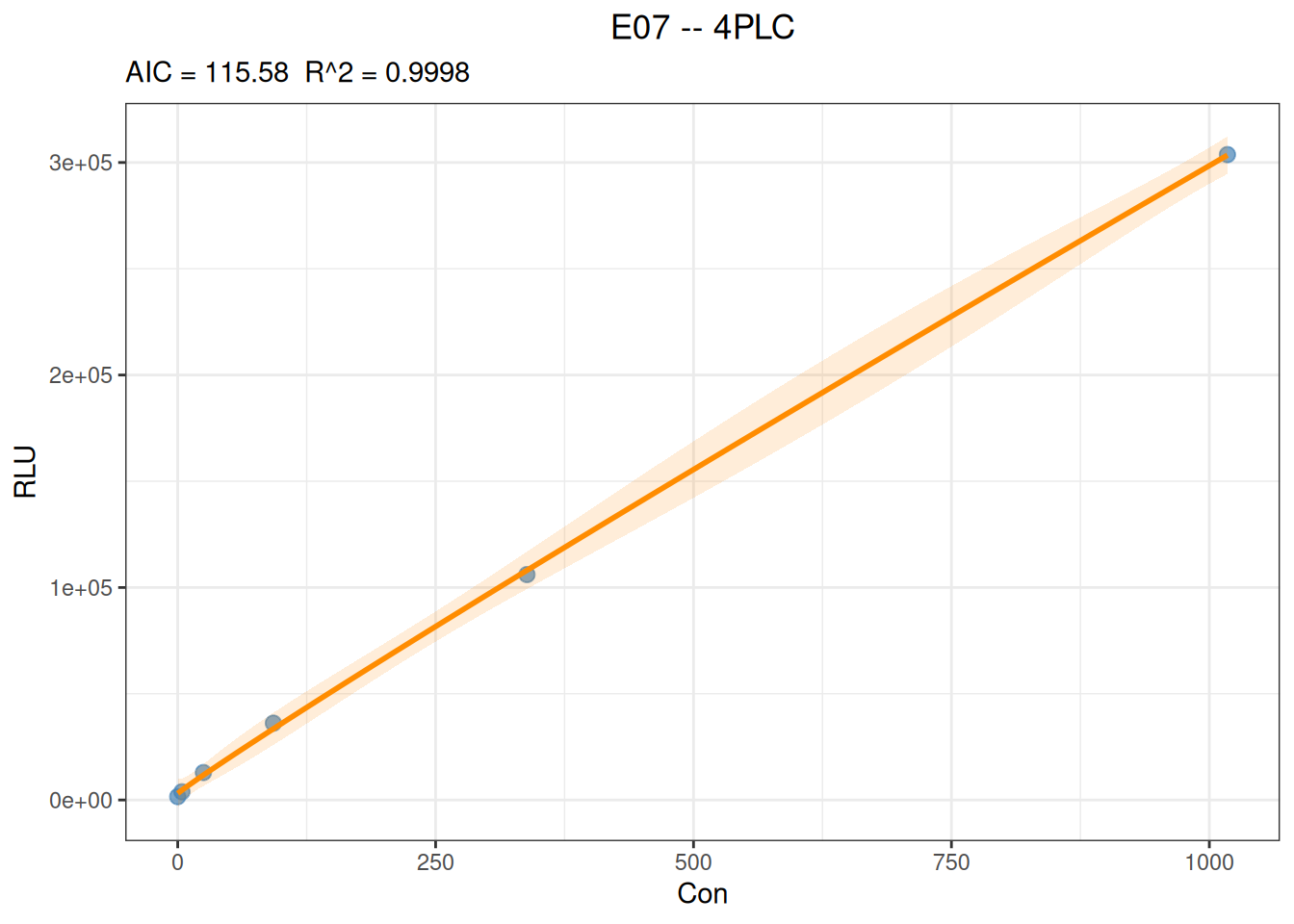

残差应同时在原始响应尺度和相对尺度上检查，并结合重复测量方差判断。对跨越多个数量级的响应，仅查看原始残差可能使高信号点主导判断。

3.3.4 由浓度预测响应

代码

predict(
  fit_u1,
  newdata = data.frame(Con = c(20, 200, 1000)),
  interval = "confidence",
  level = 0.95
)

    x         y   y_ci_lwr  y_ci_upr
   20  10095.70   5194.229  14997.17
  200  66540.68  59494.141  73587.22
 1000 298518.29 289967.527 307069.05

均值置信区间描述拟合均值的不确定性；预测区间还包含单次观测误差，通常更宽：

代码

predict(
  fit_u1,
  newdata = data.frame(Con = c(20, 200, 1000)),
  interval = "prediction",
  level = 0.95
)

    x         y      y_pi_lwr  y_pi_upr
   20  10095.70     -7.215948  20198.61
  200  66540.68  55240.318293  77841.05
 1000 298518.29 286223.575001 310813.01

3.3.5 由响应逆向估计浓度

代码

predict(
  fit_u1,
  newdata = data.frame(RLU = c(20000, 100000, 250000)),
  inverse = TRUE
)

        x      y
  50.2395  20000
 311.3672 100000
 828.5559 250000

预测边界： 应避免超出校准浓度范围外推。逆向预测在平台区对响应误差非常敏感，非单调模型还可能出现多解。当前示例拟合未可靠收敛，因此预测仅用于演示接口，不能用于定量结论。

3.4 示例二：夹心法与权重

3.4.1 等权重拟合

夹心法数据通常表现为浓度增加、信号升高。本例先进行等权重拟合：

代码

u2 <- read_csv("./data/4PLC-U2.csv", show_col_types = FALSE)

fit_u2_equal <- fit_equation(
  "4PLC",
  data = u2,
  x = "Con",
  y = "RLU"
)
print(fit_u2_equal)

E07 (4PLC)
Formula: A + (B - A) / (1 + (x / C)^D)

Call:
  fit_equation(eq = "4PLC", data = u2, x = "Con", y = "RLU")

Residuals:
      Min       1Q   Median       3Q      Max
    -1034493.852  -58331.509  17644.023  45830.410  785037.098

Coefficients:
      Estimate  Std. Error  t value   Pr(>|t|)    
A -4.19069e+04 2.74298e+05 -0.15278 0.88288329    
B  4.01980e+08 9.51404e+08  0.42251 0.68532695    
C  1.12895e+03 3.16059e+03  0.35720 0.73147078    
D -1.02539e+00 1.32241e-01 -7.75390 0.00011121 ***
---
Signif. codes:  0 '***' 0.001 '**' 0.01 '*' 0.05 '.' 0.1 ' ' 1

Residual standard error: 565331 on 7 degrees of freedom
AIC: 327.64  Iterations: 24

3.4.2 反响应平方权重拟合

当响应方差随信号增大而明显增大时，可以评估反响应平方权重：

代码

fit_u2_weighted <- fit_equation(
  "4PLC",
  data = u2,
  x = "Con",
  y = "RLU",
  weights = "1/y^2"
)
print(fit_u2_weighted)

E07 (4PLC)
Formula: A + (B - A) / (1 + (x / C)^D)

Call:
  fit_equation(eq = "4PLC", data = u2, x = "Con", y = "RLU", weights = "1/y^2")

Residuals:
      Min       1Q   Median       3Q      Max
    -1038926.254  -2031.562  491.283  35707.649  809345.965

Coefficients:
      Estimate  Std. Error    t value   Pr(>|t|)    
A  5.66828e+03 2.30614e+02   24.57907 4.7016e-08 ***
B  2.00185e+08 6.72603e+07    2.97627   0.020624 *  
C  4.83741e+02 1.74222e+02    2.77658   0.027433 *  
D -1.08082e+00 1.02400e-02 -105.54858 1.8062e-12 ***
---
Signif. codes:  0 '***' 0.001 '**' 0.01 '*' 0.05 '.' 0.1 ' ' 1

Residual standard error: 0.042025 on 7 degrees of freedom
AIC: 265.29  Iterations: 7

比较两个模型在各校准点的相对残差：

代码

u2_comparison <- data.frame(
  Sample = u2$Sample,
  Con = u2$Con,
  RLU = u2$RLU,
  Equal_weight_pct = residuals(fit_u2_equal) / u2$RLU * 100,
  Inverse_y2_weight_pct = residuals(fit_u2_weighted) / u2$RLU * 100
)
knitr::kable(u2_comparison, digits = 2)

Sample	Con	RLU	Equal_weight_pct	Inverse_y2_weight_pct
c1	0.00	5637	843.43	-0.55
c2	0.05	16014	275.49	3.07
c3	0.20	47520	67.84	-4.70
c4	0.51	125038	14.11	-1.46
c5	1.03	277621	4.57	4.70
c6	5.19	1498023	-4.39	0.98
c7	10.92	3334387	-1.53	1.70
c8	20.83	6148959	-6.53	-5.30
c9	49.90	16515788	4.75	4.13
c10	95.47	28504677	-3.63	-3.64
c11	112.18	35017203	1.75	2.31

代码

data.frame(
  Model = c("等权重", "1/y^2 权重"),
  Median_absolute_relative_residual_pct = c(
    median(abs(u2_comparison$Equal_weight_pct)),
    median(abs(u2_comparison$Inverse_y2_weight_pct))
  ),
  Maximum_absolute_relative_residual_pct = c(
    max(abs(u2_comparison$Equal_weight_pct)),
    max(abs(u2_comparison$Inverse_y2_weight_pct))
  )
) |>
  knitr::kable(digits = 2)

Model	Median_absolute_relative_residual_pct	Maximum_absolute_relative_residual_pct
等权重	4.75	843.43
1/y^2 权重	3.07	5.30

在本示例数据中，1/y^2 权重明显降低了低信号点的相对残差；这只能说明该权重更符合本数据所采用的相对误差评价目标。正式选择仍需结合各浓度重复测量的方差、回算浓度偏差、模型参数稳定性和预设接受标准。不同权重下的残差标准误和 AIC 具有不同尺度，不宜脱离误差模型直接比较。

代码

plot(fit_u2_weighted, interval = "confidence", level = 0.95)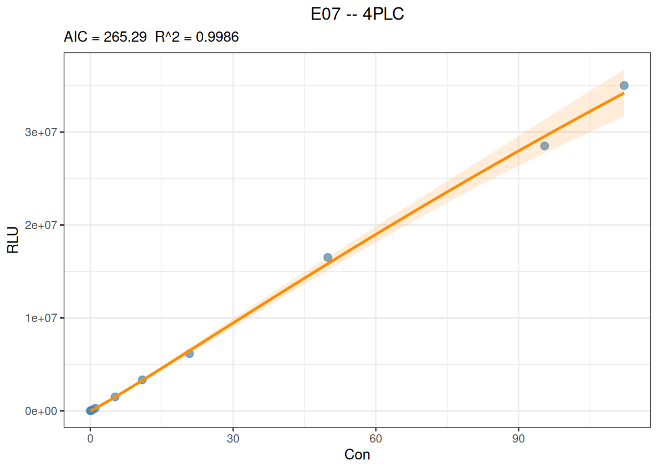

3.5 示例三：竞争法

竞争法数据通常表现为浓度增加、信号降低：

代码

u3 <- read_csv("./data/4PLC-U3.csv", show_col_types = FALSE)

fit_u3 <- fit_equation(
  "4PLC",
  data = u3,
  x = "Con",
  y = "RLU"
)
print(fit_u3)

E07 (4PLC)
Formula: A + (B - A) / (1 + (x / C)^D)

Call:
  fit_equation(eq = "4PLC", data = u3, x = "Con", y = "RLU")

Residuals:
      Min       1Q   Median       3Q      Max
    -1937.581  -454.210  -28.126  625.582  1807.765

Coefficients:
      Estimate  Std. Error   t value   Pr(>|t|)    
A -2.81576e+04 2.17005e+03  -12.9755 1.1793e-06 ***
B  1.40035e+06 1.08896e+03 1285.9562 < 2.22e-16 ***
C  1.29783e+02 6.49733e-01  199.7479 4.4162e-16 ***
D  7.82733e-01 2.79342e-03  280.2058 < 2.22e-16 ***
---
Signif. codes:  0 '***' 0.001 '**' 0.01 '*' 0.05 '.' 0.1 ' ' 1

Residual standard error: 1093.1 on 8 degrees of freedom
AIC: 207.11  Iterations: 5

代码

fit_u3$fit$convInfo[c("isConv", "finIter", "stopCode", "stopMessage")]

$isConv
[1] TRUE

$finIter
[1] 5

$stopCode
[1] 1

$stopMessage
[1] "Relative error in the sum of squares is at most `ftol'."

代码

u3_diagnostics <- data.frame(
  Sample = u3$Sample,
  Con = u3$Con,
  RLU = u3$RLU,
  Relative_residual_pct = residuals(fit_u3) / u3$RLU * 100
)
knitr::kable(u3_diagnostics, digits = 2)

Sample	Con	RLU	Relative_residual_pct
m1	0	1400548	0.01
m2	40	991716	-0.20
m3	60	897247	0.20
m4	79	822749	-0.05
m5	138	669646	0.11
m6	187	585293	0.10
m7	297	462119	-0.07
m8	523	330399	-0.19
m9	737	263095	-0.25
m10	1266	177260	-0.12
m11	1608	146827	0.11
m12	2218	112252	0.61

代码

plot(fit_u3, interval = "confidence", level = 0.95)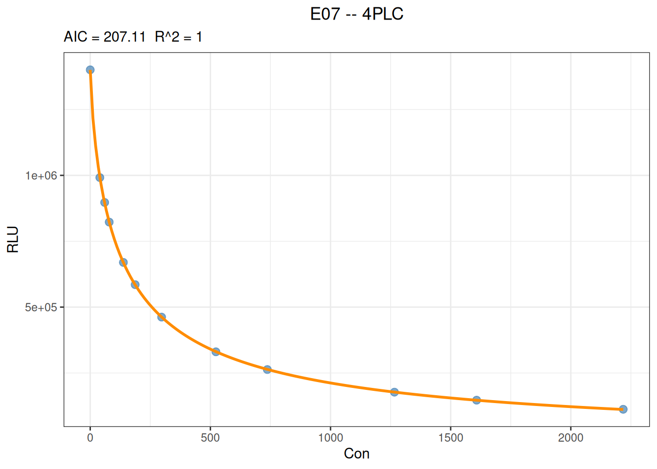

本例等权重拟合已经收敛且样本内相对残差较小，但仍应依据重复测量方差决定是否需要权重。信号方向本身不是选择等权重或加权拟合的依据。

3.6 结果判读要点

校准设计：浓度点应覆盖预期工作区间，并尽可能提供上下平台信息。
收敛状态：检查 convInfo，不能把达到最大迭代次数直接视为成功收敛。
参数合理性：结合平台、曲线中点、方向、标准误和参数相关性判断稳定性。
残差结构：同时检查原始残差、相对残差及其随浓度或拟合值的变化。
权重依据：优先使用重复测量估计的方差结构，并在分析前规定选择规则。
回算表现：按项目要求评价各校准点的回算浓度偏差和精密度。
预测范围：避免外推，尤其避免在平台区进行不稳定的逆向预测。
可复现性：保存原始数据、代码、模型参数、包版本、图形和完整会话信息。