5 精密度分析

5.1 分析目的

精密度（precision）评价同一测量系统在可重复条件下对同一样品测得结果之间的一致程度，通常用标准差（SD）或变异系数（CV%）表示。CLSI EP05 将精密度按条件细分为批内（within-run）、批间（between-run）和日间（between-day）等方差分量，并给出各分量的估计、置信区间以及用于判定的可接受限。

本文演示如何使用 ivdtools 包的 precision() 建立精密度方差分量分析，完成异常值检查、正态性评估、方差分量与置信区间估计、Sadler 精密度剖面拟合，并把结果重排为 EP05 风格的方差分量表。示例数据为确定性的教学数据，仅用于演示分析流程；正式研究必须使用方案或标准预先规定的实验设计、接受标准与分析参数。

代码

library(ivdtools)
library(readr)

数据格式要求： precision() 最终调用 VCA::anovaVCA()，要求普通 data.frame。用 readr::read_csv() 读入的是 tibble，因此本文统一先转为 data.frame，再把实验因子列（天、批、复孔等）转为因子。

5.2 函数概述

函数	主要用途	关键输入或输出
`precision()`	创建精密度方差分量分析对象	嵌套公式、`by` 分组、平衡性检查
`outlier()`	逐样本异常值检测	Grubbs 或 IQR 方法
`normal()`	逐样本正态性检验	Shapiro-Wilk 等，`level` 控制置信水平
`variance()` / `vc()`	估计方差分量	VC、%Total、SD、CV%，`NegVC` 在此传入
`ci()`	各分量 SD/CV 的置信区间	Satterthwaite 近似
`profile()`	Sadler 精密度剖面拟合	10 个候选模型、AIC 选优
`list_sadler()`	查看 10 个 Sadler 模型	模型公式与类型
`summary()` / `plot()`	汇总与绘图	`plot(type=...)` 选择图形

precision() 创建对象后，分析结果通过 outlier()、normal()、variance()、ci()、profile() 逐步累积到对象中，必须重新赋值：

precision() -> outlier() -> normal() -> variance() -> ci() -> profile()

只有已执行的分析才出现在 summary() 中，且 plot() 的某些图形依赖前置分析。

5.3 示例一：EP05 20×2×2 单样本精密度

5.3.1 读取和核验数据

20×2×2 指 20 天、每天 2 批、每批 2 个重复，共 80 个结果，是 EP05 的经典设计之一：

代码

ep05 <- read_csv("./data/precision-ep05.csv", show_col_types = FALSE)
ep05 <- as.data.frame(ep05)
str(ep05)

'data.frame':   80 obs. of  4 variables:
 $ day  : num  1 1 1 1 2 2 2 2 3 3 ...
 $ run  : num  1 1 2 2 1 1 2 2 1 1 ...
 $ rep  : num  1 2 1 2 1 2 1 2 1 2 ...
 $ value: num  96.9 93.5 99.3 101.5 103 ...

实验因子列在 CSV 中为整数，读取后转换为因子：

代码

ep05$day <- factor(ep05$day)
ep05$run <- factor(ep05$run)
ep05$rep <- factor(ep05$rep)

代码

dim(ep05)

[1] 80  4

代码

summary(ep05$value)

   Min. 1st Qu.  Median    Mean 3rd Qu.    Max. 
  86.06   94.83   99.33   99.11  103.53  115.01

value ~ day/run 表示方差分量按日间（day）→ 日内的批（run）逐层嵌套。 / 是嵌套记法，等价于把每个深一层因子视为上一层因子的分组内因子。

5.3.2 创建分析对象并预检

代码

p <- precision(ep05, value ~ day/run)
p

Precision analysis object
  Data class          : data.frame
  Total rows          : 80
  Formula             : value ~ day/run
  Samples             : 1

Factor levels
  day         : 1 (4), 2 (4), 3 (4), 4 (4), 5 (4), 6 (4), 7 (4), 8 (4), 9 (4), 10 (4), 11 (4), 12 (4), 13 (4), 14 (4), 15 (4), 16 (4), 17 (4), 18 (4), 19 (4), 20 (4)
  run         : 1 (40), 2 (40)
  rep         : 1 (40), 2 (40)

Analysis status

  [ ] outlier
  [ ] normal
  [ ] variance
  [ ] ci
  [ ] profile

平衡性检查输出提示最大/最小单元大小之比；当数据高度不平衡时，VCA 会提示改用 REML。

逐样本做异常值检测和正态性检验：

代码

p <- outlier(p, method = "grubbs")

Outlier detection -- Grubbs (alpha = 0.05)
  No outliers detected.

代码

p <- normal(p, method = "shapiro")

Normality test -- Shapiro-Wilk
  Sample               n           W  p-value
  ---------------------------------------------
  all                 80      0.9868  0.5858

参数说明： outlier() 的 method 可选 "grubbs"（默认）或 "iqr"，alpha 为 Grubbs 显著性水平。normal() 的 method="auto" 会根据样本量选择检验（n≤50 用 Shapiro-Wilk、更大用 Anderson-Darling 等）；指定 method="shapiro" 时输出的 W 列才是真正的 Shapiro-Wilk W 统计量。单样本数据 n=80，两种方式均可接受，本示例显式指定以便展示。

5.3.3 方差分量与置信区间

代码

p <- variance(p)

Variance components
 sample component      VC %Total     SD  CV[%]
----------------------------------------------
    all       day 18.8358   42.6 4.3400 4.3788
    all   day:run 17.4343   39.4 4.1754 4.2128
    all     error  7.9482   18.0 2.8193 2.8445

NegVC 参数需要在 variance() 处传入：

代码

p <- variance(p, NegVC = TRUE)   # 允许负方差分量（默认 FALSE）

代码

p <- ci(p)

Confidence intervals (SD)
 sample component estimate  lower  upper
----------------------------------------
    all     total   6.6497 5.4288 8.5842
    all       day   4.3400 0.0000 6.2255
    all   day:run   4.1754 2.0129 5.5513
    all     error   2.8193 2.3147 3.6073 

Confidence intervals (%CV)
 sample component estimate  lower  upper
----------------------------------------
    all     total   6.7091 5.4773 8.6609
    all       day   4.3788 0.0000 6.2812
    all   day:run   4.2128 2.0309 5.6009
    all     error   2.8445 2.3353 3.6395

ci() 采用 Satterthwaite 有效自由度近似计算各分量 SD 与 CV 的置信区间。

5.3.4 转化为 EP05 术语表

按分量名的嵌套深度把方差分量归入批内、批间、日间，并计算总 SD/CV，进一步把各分量置信区间合并形成带区间的完整 EP05 报告表。统计结果是否可接受必须依据方案预先规定的精密度限值判定。

5.3.5 图形

散点图可用于快速识别测试异常和测值分布情况：

代码

plot(p, type = "dot")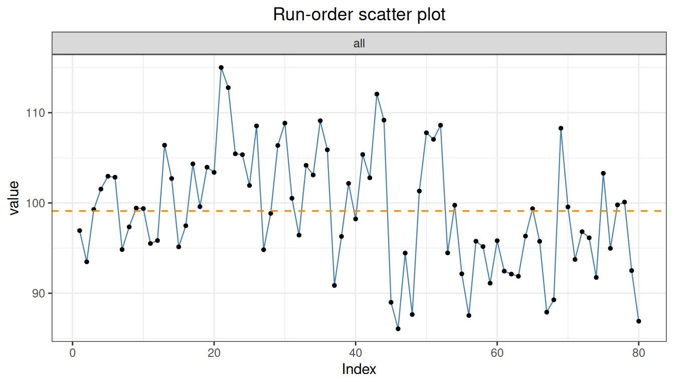

代码

plot(p, type = "qq")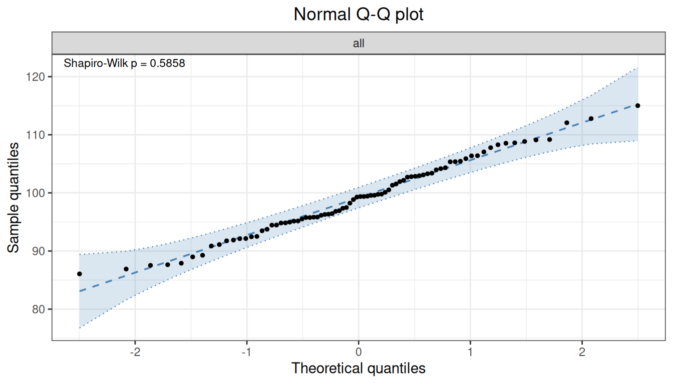

图形依赖： plot(type="dot") 为按运行顺序的散点（无需前置分析），type="his" 为标准直方图； type="var" 需要先执行 variance()，type="qq" 需要先执行 normal()，type="profile" 需要先执行 profile()。绘图前请确认对应分析已运行。

代码

summary(p)


Precision analysis -- summary
---------------------------------------- 

Precision analysis object
  Data class          : data.frame
  Total rows          : 80
  Formula             : value ~ day/run
  Samples             : 1

Factor levels
  day         : 1 (4), 2 (4), 3 (4), 4 (4), 5 (4), 6 (4), 7 (4), 8 (4), 9 (4), 10 (4), 11 (4), 12 (4), 13 (4), 14 (4), 15 (4), 16 (4), 17 (4), 18 (4), 19 (4), 20 (4)
  run         : 1 (40), 2 (40)
  rep         : 1 (40), 2 (40)

Analysis status

  [x] outlier
  [x] normal
  [x] variance
  [x] ci
  [ ] profile

Outlier detection -- Grubbs (alpha = 0.05)
  No outliers detected.

Normality test -- Shapiro-Wilk
  Sample               n           W  p-value
  ---------------------------------------------
  all                 80      0.9868  0.5858

Variance components
 sample component      VC %Total     SD  CV[%]
----------------------------------------------
    all       day 18.8358   42.6 4.3400 4.3788
    all   day:run 17.4343   39.4 4.1754 4.2128
    all     error  7.9482   18.0 2.8193 2.8445 

Confidence intervals (SD)
 sample component estimate  lower  upper
----------------------------------------
    all     total   6.6497 5.4288 8.5842
    all       day   4.3400 0.0000 6.2255
    all   day:run   4.1754 2.0129 5.5513
    all     error   2.8193 2.3147 3.6073 

Confidence intervals (%CV)
 sample component estimate  lower  upper
----------------------------------------
    all     total   6.7091 5.4773 8.6609
    all       day   4.3788 0.0000 6.2812
    all   day:run   4.2128 2.0309 5.6009
    all     error   2.8445 2.3353 3.6395

5.4 示例二：多样本3×5与 Sadler 剖面

5.4.1 读取数据

当需要评价多个浓度水平时，用 by 指定样本分组列，各样本分别估计方差分量：

代码

profile_data <- as.data.frame(read_csv(
  "./data/precision-profile.csv",
  show_col_types = FALSE
))
profile_data$sample <- factor(profile_data$sample)
profile_data$day <- factor(profile_data$day)
profile_data$rep <- factor(profile_data$rep)

5.4.2 样本方差分量

代码

p2 <- precision(profile_data, value ~ day, by = "sample")
p2 <- variance(p2)

Variance components
 sample component       VC %Total      SD  CV[%]
------------------------------------------------
     L1       day   0.6376   63.0  0.7985 3.9446
     L1     error   0.3750   37.0  0.6124 3.0250
     L2       day   5.7139   75.1  2.3904 4.7584
     L2     error   1.8937   24.9  1.3761 2.7393
     L3       day   3.3913   15.7  1.8415 1.8088
     L3     error  18.1466   84.3  4.2599 4.1840
     L4       day  30.5549   54.6  5.5276 2.7529
     L4     error  25.4525   45.4  5.0451 2.5126
     L5       day   0.0000    0.0  0.0000 0.0000
     L5     error 171.7986  100.0 13.1072 3.3003

代码

p2 <- ci(p2)

Confidence intervals (SD)
 sample component estimate  lower   upper
-----------------------------------------
     L1     total   1.0063 0.6007  2.9368
     L1       day   0.7985 0.0000  1.4267
     L1     error   0.6124 0.4391  1.0108
     L2     total   2.7582 1.5714  9.9889
     L2       day   2.3904 0.0000  4.2023
     L2     error   1.3761 0.9868  2.2716
     L3     total   4.6409 3.2872  7.8819
     L3       day   1.8415 0.0000  4.1779
     L3     error   4.2599 3.0547  7.0319
     L4     total   7.4838 4.6166 19.1652
     L4       day   5.5276 0.0000 10.0268
     L4     error   5.0451 3.6177  8.3280
     L5     total  13.1072 9.5629 20.8255
     L5       day   0.0000     NA      NA
     L5     error  13.1072 9.3990 21.6365 

Confidence intervals (%CV)
 sample component estimate  lower   upper
-----------------------------------------
     L1     total   4.9710 2.9673 14.5079
     L1       day   3.9446 0.0000  7.0480
     L1     error   3.0250 2.1692  4.9936
     L2     total   5.4905 3.1281 19.8843
     L2       day   4.7584 0.0000  8.3652
     L2     error   2.7393 1.9643  4.5219
     L3     total   4.5583 3.2287  7.7416
     L3       day   1.8088 0.0000  4.1035
     L3     error   4.1840 3.0003  6.9067
     L4     total   3.7271 2.2992  9.5447
     L4       day   2.7529 0.0000  4.9936
     L4     error   2.5126 1.8017  4.1476
     L5     total   3.3003 2.4078  5.2436
     L5       day   0.0000     NA      NA
     L5     error   3.3003 2.3666  5.4478

比较样本的变异比例，可用于产品优化和检验方案设计：

代码

plot(p2, type = "var")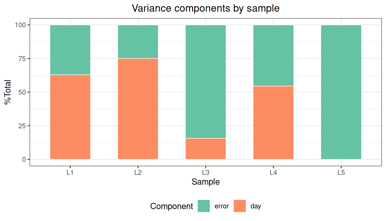

5.4.3 精密度剖面

profile() 对每个方差分量拟合 Sadler 模型族，按 AIC 选出最优模型：

代码

list_sadler()

Sadler Precision Profile Models

   1  Constant SD           sigma^2 = b1
   2  Constant CV           sigma^2 = b1 * mu^2
   3  Linear (variance)     sigma^2 = b1 + b2 * mu
   4  Power (fixed K)       sigma^2 = b1 * mu^K
   5  Power (fixed K, +intercept)  sigma^2 = b1 + b2 * mu^K
   6  Linear (SD)           sigma = b1 + b2 * mu
   7  Power (SD)            sigma = b1 + b2 * mu^b3
   8  Power (variance)      sigma^2 = b1 + b2 * mu^b3
   9  Exponential (log-log)  log(sigma^2) = b1 + b2 * log(mu)
  10  Power (full)          sigma^2 = b1 * mu^b2

代码

p2 <- profile(p2, model.no = 1:10)

Precision profiles -- Sadler
  total: sigma = 0.0000 + 0.0086 * mu^1.6702  (AIC = 56.45, R^2 = 0.9847)
  day: sigma = 0.0000 + 0.0095 * mu^1.4951  (AIC = 43.46, R^2 = 0.8919)
  error: sigma^2 = 0.0010 * mu^2  (AIC = 55.96, R^2 = 0.9806)

代码

plot(p2, type = "profile")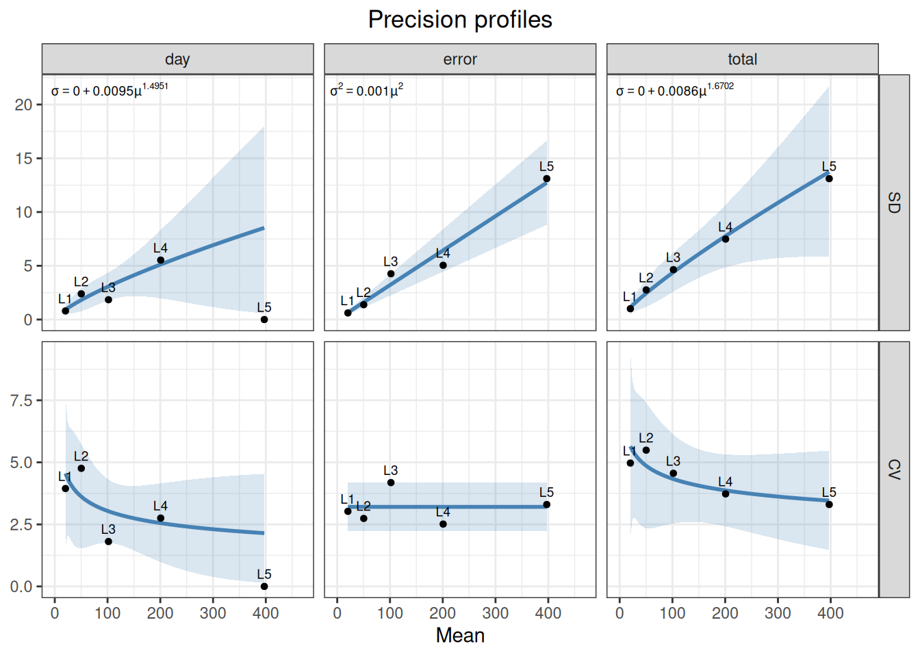

参数说明： profile(model.no = 1:10) 指定候选模型序号；... 可传给内部 Sadler 拟合（例如 K）。每个方差分量至少需要 3 个样本具有有限 SD 才能拟合，因此多样本设计至少应设 3 个浓度水平。剖面可用于功能灵敏度等分析中预测任意浓度下的 SD/CV（参见《功能灵敏度》）。

本示例 total 与 day 分量最优模型为幂函数型（模型 7），day:rep 分量为恒定 CV 型（模型 2），符合”SD 随浓度升高而增大、CV 相对稳定”的常见设定。

5.5 示例三：多样本多中心（站点）精密度

5.5.1 读取数据

数据包含 2 个站点（site）、3 个样本（sample），每站点每样本 3 天 × 3 批 × 5 复孔：

代码

sites_data <- as.data.frame(read_csv(
  "./data/precision-sites.csv",
  show_col_types = FALSE
))
sites_data[] <- lapply(sites_data, function(x)
  if (is.numeric(x) && all(x == round(x))) factor(x) else x)
str(sites_data)

'data.frame':   270 obs. of  6 variables:
 $ site  : chr  "A" "A" "A" "A" ...
 $ sample: chr  "S1" "S1" "S1" "S1" ...
 $ day   : Factor w/ 3 levels "1","2","3": 1 1 1 1 1 1 1 1 1 1 ...
 $ run   : Factor w/ 3 levels "1","2","3": 1 1 1 1 1 2 2 2 2 2 ...
 $ rep   : Factor w/ 5 levels "1","2","3","4",..: 1 2 3 4 5 1 2 3 4 5 ...
 $ value : num  49.2 52.3 48.8 49.4 51.5 ...

5.5.2 多列分组

by 可接受多个列名，内部按交互作用分组，一次得到所有站点 × 样本组合：

代码

p3 <- precision(sites_data, value ~ day/run, by = c("sample", "site"))
p3 <- variance(p3)

Variance components
 sample component      VC %Total     SD  CV[%]
----------------------------------------------
   S1.A       day  0.0000    0.0 0.0000 0.0000
   S1.A   day:run  0.1646    6.8 0.4057 0.8231
   S1.A     error  2.2677   93.2 1.5059 3.0553
   S2.A       day  0.3241    4.3 0.5693 0.5602
   S2.A   day:run  0.1523    2.0 0.3903 0.3840
   S2.A     error  7.0483   93.7 2.6549 2.6124
   S3.A       day  4.4871   15.6 2.1183 1.0420
   S3.A   day:run  1.7006    5.9 1.3041 0.6415
   S3.A     error 22.5797   78.5 4.7518 2.3375
   S1.B       day  0.0000    0.0 0.0000 0.0000
   S1.B   day:run  0.5459   23.5 0.7389 1.4758
   S1.B     error  1.7784   76.5 1.3335 2.6637
   S2.B       day  0.0000    0.0 0.0000 0.0000
   S2.B   day:run  1.6690   21.5 1.2919 1.2891
   S2.B     error  6.0856   78.5 2.4669 2.4616
   S3.B       day  0.7633    2.3 0.8737 0.4448
   S3.B   day:run  0.0000    0.0 0.0000 0.0000
   S3.B     error 31.8033   97.7 5.6394 2.8709

代码

names(p3$results)

[1] "S1.A" "S2.A" "S3.A" "S1.B" "S2.B" "S3.B"

5.5.3 按站点拆分单独分析

等价的做法是先按站点 split()，再对每个站点子集执行相同的分析参数。当站点间的方差分量结构预计不同，或需要分别出具报告时，拆分后单独分析更清晰：

代码

for (s in c("A", "B")) {
  sub <- sites_data[sites_data$site == s, ]
  ps <- precision(sub, value ~ day/run, by = "sample")
  ps <- variance(ps)
  ps <- ci(ps)
}

注意： 多中心研究应统一分析方案、方差分量模型与报告口径；“先按中心出报告、再合并汇总” 时，务必记录每个中心的原始数据是否纳入、排除标准与因子定义是否一致。

5.6 示例四：自定义的更复杂模型

5.6.1 读取数据

除标准的天/批/重复嵌套外，precision() 的公式可以是任意 VCA 嵌套结构，例如再加入操作者（operator）层：value ~ operator/day/run，即操作者 → 天 → 批逐层嵌套：

代码

custom_data <- as.data.frame(read_csv(
  "./data/precision-custom.csv",
  show_col_types = FALSE
))
custom_data[] <- lapply(custom_data, function(x)
  if (is.numeric(x) && all(x == round(x))) factor(x) else x)

5.6.2 拟合与解读

代码

p4 <- precision(custom_data, value ~ operator/day/run)
p4 <- variance(p4)

Variance components
 sample        component     VC %Total     SD  CV[%]
----------------------------------------------------
    all         operator 2.2914   11.8 1.5137 1.4898
    all     operator:day 6.3159   32.4 2.5132 2.4734
    all operator:day:run 3.2463   16.7 1.8017 1.7733
    all            error 7.6322   39.2 2.7627 2.7190

5.7 结果判读要点

设计匹配：先明确研究设计的嵌套结构，precision() 的公式要如实反映实验分层。
数据格式：read_csv 读取后转 data.frame，因子列显式转 factor，避免 VCA 报错或歧义。
调用顺序：outlier → normal → variance → ci → profile，每次分析重新赋值；绘图依赖前置分析。
负分量：某层因子水平过少或数据恰好相近时方差分量会被归零，需谨慎解释并在方案中规定处理方式。
CI 适用性：Satterthwaite 近似在方差分量很少或不平衡时准确性下降，报告时注明方法。
术语表：把 $results 的数值量（sd_comp/cv_comp/vc）重排为 EP05 术语表，不要直接使用展示用字符串 $vc。
可接受判定：统计估计不自动构成合格判定，应与预设精密度限值比较，并由专业人员复核。