6 线性分析

6.1 分析目的

线性（linearity）评价测量系统在整个工作范围内，测得结果与被测物浓度（或目标量值）之间是否存在可接受的线性关系，通常采用稀释数据，按 CLSI EP06 分析偏差。本文演示如何使用 ivdtools 包的 fit_equation() 完成线性拟合、加权拟合、各水平偏差与残差评价，以及使用 fit_equation() 做 EP06-A2 风格的多项式分析，判断是否需要引入高次项。

示例数据为确定性的教学数据，仅用于演示流程；正式研究应使用方案中预先规定的稀释方案、浓度水平、重复数与接受标准。

代码

library(ivdtools)
library(readr)

6.2 函数概述

函数	主要用途	关键输入或输出
`list_equation()`	查看内置方程注册表	`category`、`engine` 过滤
`replicate_to_mean()`	汇总重复测量并可计算权重	`"n"`、`"1/sd"`、`"1/sd^2"`
`fit_equation()`	拟合内置或自定义方程	`eq`、`weights`、`lower/upper`、`constraints`
`compare_equation()`	拟合多个候选方程并按 AIC 排序	`eqs`、deltaAIC
`coef()` / `residuals()`	提取参数与残差
`predict()`	正向预测或逆向回算浓度	`inverse=TRUE`、`interval`
`plot()`	绘制拟合曲线与区间	`interval`、`frame`

6.3 示例一：系列稀释的线性偏差

6.3.1 读取和核验数据

稀释系列包含 8 个浓度水平、每水平 3 次重复，共 24 行：

代码

dilution <- read_csv("./data/linearity-dilution.csv", show_col_types = FALSE)
dilution <- as.data.frame(dilution)
head(dilution, 6)

代码

dim(dilution)

[1] 24  3

代码

summary(dilution)

      conc        replicate     signal      
 Min.   :  50   Min.   :1   Min.   :  48.6  
 1st Qu.: 175   1st Qu.:1   1st Qu.: 173.6  
 Median : 600   Median :2   Median : 595.6  
 Mean   :1594   Mean   :2   Mean   :1593.0  
 3rd Qu.:2000   3rd Qu.:3   3rd Qu.:2004.5  
 Max.   :6400   Max.   :3   Max.   :6406.9

6.3.2 查看可用响应方程

代码

list_equation(category = "Response")

  ID       Name                         Formula        Params nP Engine
-----------------------------------------------------------------------
 E01     Linear                         a + b*x          a, b  2     lm
 E02  Quadratic                 a + b*x + c*x^2       a, b, c  3     lm
 E03 ExpoGrowth                  a * exp(b * x)          a, b  2    nls
 E04  ExpoDecay                 a * exp(-b * x)          a, b  2    nls
 E05      Power                         a * x^b          a, b  2    nls
 E06        Log                  a + b * log(x)          a, b  2     lm
 E07       4PLC   A + (B - A) / (1 + (x / C)^D)    A, B, C, D  4    nls
 E08       5PLC A + (B - A) / (1 + (x / C)^D)^E A, B, C, D, E  5    nls
 E09   Gaussian a * exp(-(x - b)^2 / (2 * c^2))       a, b, c  3    nls
 E10  Michaelis             Vmax * x / (Km + x)      Vmax, Km  2    nls
 E11 Sinusoidal          a * sin(b * x + c) + d    a, b, c, d  4    nls
 E12      Cubic         a + b*x + c*x^2 + d*x^3    a, b, c, d  4     lm

线性方程对应注册表 ID E01（也接受名称 "Linear"）。

6.3.3 汇总重复测量

先使用 replicate_to_mean() 得到每水平均值、SD 与重复数。

代码

rep_sum <- replicate_to_mean(dilution, x = "conc", y = "signal")
rep_sum

6.3.4 线性拟合与偏差

代码

fit_lin <- fit_equation("E01", data = rep_sum, x = "x", y = "y_mean")
print(fit_lin)

E01 (Linear)
Formula: a + b*x

Call:
  stats::lm(formula = frm, data = d, weights = weights)

Residuals:
      Min       1Q   Median       3Q      Max
    -4.330   -2.404   -1.439    0.430   10.364

Coefficients:
  Estimate  Std. Error    t value Pr(>|t|)    
a 0.975290 2.205878722    0.44213  0.67388    
b 0.998894 0.000844269 1183.14720  < 2e-16 ***
---
Signif. codes:  0 '***' 0.001 '**' 0.01 '*' 0.05 '.' 0.1 ' ' 1

Residual standard error: 4.944 on 6 degrees of freedom
Multiple R-squared: 1.0000,  Adjusted R-squared: 1.0000
F-statistic: 1.39984e+06 on 1 and 6 DF,  p-value: <2e-16

计算原始残差即线性偏差（实测均值与预测值）与回收偏差（实测均值与理论值）：

代码

predict <- predict(fit_lin)

    x          y
   50   50.91999
  100  100.86468
  200  200.75408
  400  400.53286
  800  800.09044
 1600 1599.20559
 3200 3197.43588
 6400 6393.89648

代码

lin_diag <- data.frame(
  conc = rep_sum$x,
  signal = rep_sum$y_mean,
  predict = predict$y,
  Residual = residuals(fit_lin),
  Recover_bias = rep_sum$y_mean - rep_sum$x
)
print(lin_diag)

  conc     signal    predict    Residual Recover_bias
1   50   49.26667   50.91999 -1.65332058   -0.7333333
2  100  100.80000  100.86468 -0.06468401    0.8000000
3  200  202.66667  200.75408  1.91258912    2.6666667
4  400  397.83333  400.53286 -2.69953130   -2.1666667
5  800  798.86667  800.09044 -1.22377212   -1.1333333
6 1600 1596.90000 1599.20559 -2.30558710   -3.1000000
7 3200 3207.80000 3197.43588 10.36411628    7.8000000
8 6400 6389.56667 6393.89648 -4.32981030  -10.4333333

偏差是否可接受须与方案中预先规定的线性接受限比较。

参数说明： fit_equation() 的 weights 接受数值向量或内置方案 "equal"、"1/y"、"1/y^2"、 "1/x"、"1/x^2"、"inverse"、"inverse2"。加权与等权重的拟合都应结合残差结构、回算偏差和预设接受标准综合比较，不能单看某一条拟合指标。

6.3.5 图形与预测

代码

plot(fit_lin, interval = "confidence", level = 0.95)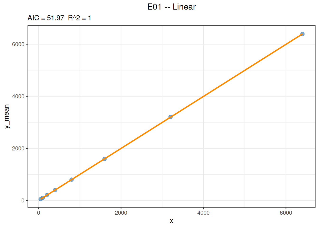

代码

predict(
  fit_lin,
  newdata = data.frame(x = c(0.5, 2, 8)),
  interval = "confidence"
)

   x        y  y_ci_lwr  y_ci_upr
 0.5 1.474737 -3.922223  6.871698
 2.0 2.973078 -2.421993  8.368150
 8.0 8.966442  3.578916 14.353968

由响应逆向回算浓度：

代码

predict(
  fit_lin,
  newdata = data.frame(y_mean = c(650, 3300, 6500)),
  inverse = TRUE
)

         x    y
  649.7434  650
 3302.6777 3300
 6506.2210 6500

预测边界： 逆向回算应避免超出校准浓度范围外推。线性模型在范围内回算是稳定的，但在平台或非线性区间，逆向预测对响应误差非常敏感。

6.4 示例二：对半稀释的多项式分析

6.4.1 读取和核验数据

数据为 5 个浓度水平 × 3 复孔：

代码

poly_data <- read_csv("./data/linearity-polynomial.csv", show_col_types = FALSE)
poly_data <- as.data.frame(poly_data)
head(poly_data, 6)

6.4.2 计算重复测试均值，并引入权重：

代码

rep_sum_w <- replicate_to_mean(
  poly_data,
  x = "conc",
  y = "signal",
  weights = "1/sd^2"
)
rep_sum_w

参数说明： replicate_to_mean() 的 weights 可选 NULL（不生成权重列）、"n"、 "1/sd" 或 "1/sd^2"（反方差加权）。权重应依据重复测量的实际方差结构或方案确定。

6.4.3 候选方程比较

EP06-A2 通常比较线性、二次、三次模型，判断是否需要高次项并比较 Residual standard error：

代码

fit_poly_lin <- fit_equation("E01", data = rep_sum_w, x = "x", y = "y_mean", weights = rep_sum_w$weights)
print(fit_poly_lin)

E01 (Linear)
Formula: a + b*x

Call:
  stats::lm(formula = frm, data = d, weights = weights)

Residuals:
      Min       1Q   Median       3Q      Max
    -20.993  -17.367   -5.447   16.760   27.047

Coefficients:
   Estimate Std. Error  t value   Pr(>|t|)    
a -18.00771 20.0633790 -0.89754    0.43557    
b   1.01397  0.0188681 53.73983 1.4192e-05 ***
---
Signif. codes:  0 '***' 0.001 '**' 0.01 '*' 0.05 '.' 0.1 ' ' 1

Residual standard error: 24.3886 on 3 degrees of freedom
Multiple R-squared: 0.9990,  Adjusted R-squared: 0.9986
F-statistic: 2887.97 on 1 and 3 DF,  p-value: 1.42e-05

代码

fit_poly_qua <- fit_equation("E02", data = rep_sum_w, x = "x", y = "y_mean", weights = rep_sum_w$weights)
print(fit_poly_qua)

E02 (Quadratic)
Formula: a + b*x + c*x^2

Call:
  stats::lm(formula = frm, data = d, weights = weights)

Residuals:
      Min       1Q   Median       3Q      Max
    -13.443  -13.294  -13.146    8.912   30.970

Coefficients:
      Estimate  Std. Error t value  Pr(>|t|)   
a -7.14812e+00 3.09846e+01 -0.2307 0.8389994   
b  9.72049e-01 8.28550e-02 11.7319 0.0071872 **
c  2.34851e-05 4.48020e-05  0.5242 0.6524439   
---
Signif. codes:  0 '***' 0.001 '**' 0.01 '*' 0.05 '.' 0.1 ' ' 1

Residual standard error: 28.0077 on 2 degrees of freedom
Multiple R-squared: 0.9991,  Adjusted R-squared: 0.9982
F-statistic: 1095.05 on 2 and 2 DF,  p-value: 0.000912

代码

fit_poly_cub <- fit_equation("E12", data = rep_sum_w, x = "x", y = "y_mean", weights = rep_sum_w$weights)
print(fit_poly_cub)

E12 (Cubic)
Formula: a + b*x + c*x^2 + d*x^3

Call:
  stats::lm(formula = frm, data = d, weights = weights)

Residuals:
      Min       1Q   Median       3Q      Max
    -13.146   -2.191   -2.191    8.764    8.764

Coefficients:
      Estimate  Std. Error  t value Pr(>|t|)
a  2.04822e+01 2.48863e+01  0.82303  0.56161
b  7.25244e-01 1.39796e-01  5.18788  0.12123
c  3.86253e-04 1.91646e-04  2.01544  0.29321
d -1.35487e-07 7.07339e-08 -1.91545  0.30631

Residual standard error: 18.3308 on 1 degrees of freedom
Multiple R-squared: 0.9998,  Adjusted R-squared: 0.9992
F-statistic: 1705.48 on 3 and 1 DF,  p-value: 0.0178

6.5 结果判读要点

拟合与模型判断分开：模型可被成功拟合不代表模型适用，应结合残差、偏差、接受标准与方案判断。
残差双尺度：同时检查原始残差与相对残差；跨数量级数据以相对残差为主。
权重依据：优先用重复测量的方差结构或方案规定。
范围与外推：结论只在验证的浓度范围内有效；逆向预测避免在平台区或范围外进行。
可复现性：保存原始数据、代码、模型参数、收敛信息、包版本与完整会话信息。