代码
library(ivdtools)
library(readr)分析灵敏度(analytical sensitivity)描述测量系统在低浓度端区分”信号与噪声”的能力,由三个递进的 限值构成:
本文演示如何使用 ivdtools 包的 lob_lod_loq() 依据 CLSI EP17-A2 计算分析灵敏度:
LoB = M_B + cp·SD_B,将全部空白结果合并为池,cp = 1.645/√(1 − 1/(4(B−K))) 为小样本修正的 95% 单侧分位数(B 为空白结果总数、K 为空白样本数)。X = LoB + cp·SD_WL(X),cp = 1.645/√(1 − 1/(4(N_TOT−K)))。√Var(X)/X = target_cv。该 LoQ 仅反映精密度、不含偏差。示例数据为确定性的教学数据,仅用于演示流程;正式研究必须依据方案或标准预先规定的实验设计、 目标浓度与接受标准。
library(ivdtools)
library(readr)| 函数 | 主要用途 | 关键输入或输出 |
|---|---|---|
lob_lod_loq() |
一次计算 LoB / LoD / LoQ | 汇总数据、空白样本名、目标 CV |
replicate_to_mean() |
汇总重复测量 | 均值、SD、重复数 n |
fit_equation() |
拟合 Sadler 精度轮廓(内部调用) | eq="sadler"、df_col |
print() / plot() |
结果展示 | 表格式汇总、SD/CV 双面板 |
lob_lod_loq() 的输入是已汇总的 data.frame:每行一个样本,含样本名称列、均值列(即浓度)、 SD 列与重复数 n 列,列名可自由指定。它内部自动完成 Sadler 最优模型拟合,无需用户手动拟合。
数据包含 2 个空白样本(blank_A、blank_B)与 6 个低浓度样本(L1–L6),各样本重复测量 (空白各 40 次、低浓度各 30 次),共 260 行。SD 随浓度升高而增大,符合低浓度端”方差随均值增大”的常见情形:
sens <- read_csv("./data/sensitivity.csv", show_col_types = FALSE)
sens <- as.data.frame(sens)
str(sens)
'data.frame': 260 obs. of 2 variables:
$ sample: chr "blank_A" "blank_A" "blank_A" "blank_A" ...
$ value : num 0.024 -0.006 0.055 -0.072 0.057 -0.023 -0.05 0.003 0.051 0.029 ...dim(sens)[1] 260 2table(sens$sample)
blank_A blank_B      L1      L2      L3      L4      L5      L6
40 40 30 30 30 30 30 30 用 replicate_to_mean() 按样本名称分组计算均值、SD 与重复数(分组变量为字符时保留原值, 两个空白各占一行):
rep <- replicate_to_mean(data.frame(x = sens$sample, y = sens$value),
                         x = "x", y = "y")
rep$sample <- rep$x
rep$mean   <- rep$y_mean
rep$sd     <- rep$y_sd
rep$n      <- rep$y_n
rep[c("sample", "mean", "sd", "n")]
注意:
lob_lod_loq()要求方差模型响应为方差、并按自由度加权,因此汇总后还需给每行补var = sd^2与df = n − 1两列,再交给lob_lod_loq()。若你的数据已含这两列则无需此步。
blank 参数指定空白样本名称(可多个),target_cv 指定 LoQ 的精密度目标:
summ <- rep[c("sample", "mean", "sd", "n")]
res <- lob_lod_loq(summ, sample_col = "sample", mean_col = "mean",
                   sd_col = "sd", n_col = "n",
                   blank = c("blank_A", "blank_B"), target_cv = 0.20)
res
Limit of Blank / Detection / Quantitation (EP17-A2)
Precision profile: Sadler; best model = Model_3
Equation : sigma^2 = b1 + b2 * mu^2
Parameters : b1 = 0.010196, b2 = 0.010388
Fit : AIC = -479.4; RSS = 0.08315; GoF p = 0.9437
LoB (parametric, B = 80, K = 2) : 0.08357
LoD (fixed-point) : 0.2552
LoQ (CV = 20%) : 0.5868
Note: LoQ is based on precision ONLY; bias is not included.结果解读:
X = LoB + cp·SD(X) 的固定点,即高于此浓度的测值可判为”非空白”。lob_lod_loq() 返回 sensitivity 对象,各限值与参数以命名分量保存:
str(res, max.level = 1)List of 13
$ call : language lob_lod_loq(data = summ, sample_col = "sample", mean_col = "mean", sd_col = "sd", n_col = "n", blank = c("bl| __truncated__
$ lob : num 0.0836
$ lod : num 0.255
$ loq : num 0.587
$ n_blank : int 80
$ B : int 80
$ K : int 2
$ target_cv: num 0.2
$ cp_lob : num 1.65
$ cp_lod : num 1.65
$ fit :List of 12
..- attr(*, "class")= chr "fit_equation"
$ model : chr "Model_3"
$ notes : chr(0)
- attr(*, "class")= chr "sensitivity"res$lob[1] 0.0835705res$lod[1] 0.2552205res$loq[1] 0.5867594res$B[1] 80res$K[1] 2res$cp_lob[1] 1.647643res$cp_lod[1] 1.646183res$model[1] "Model_3"cp_lob、cp_lod 即 EP17 的两个小样本修正系数;model 为 AIC 选出的最优 Sadler 模型 (本例为模型 3,混合方差型)。
plot() 画出 SD 与 CV 两个精度轮廓面板,叠加 LoB / LoD / LoQ 参考线,直观展示各限值的 几何含义:
plot(res)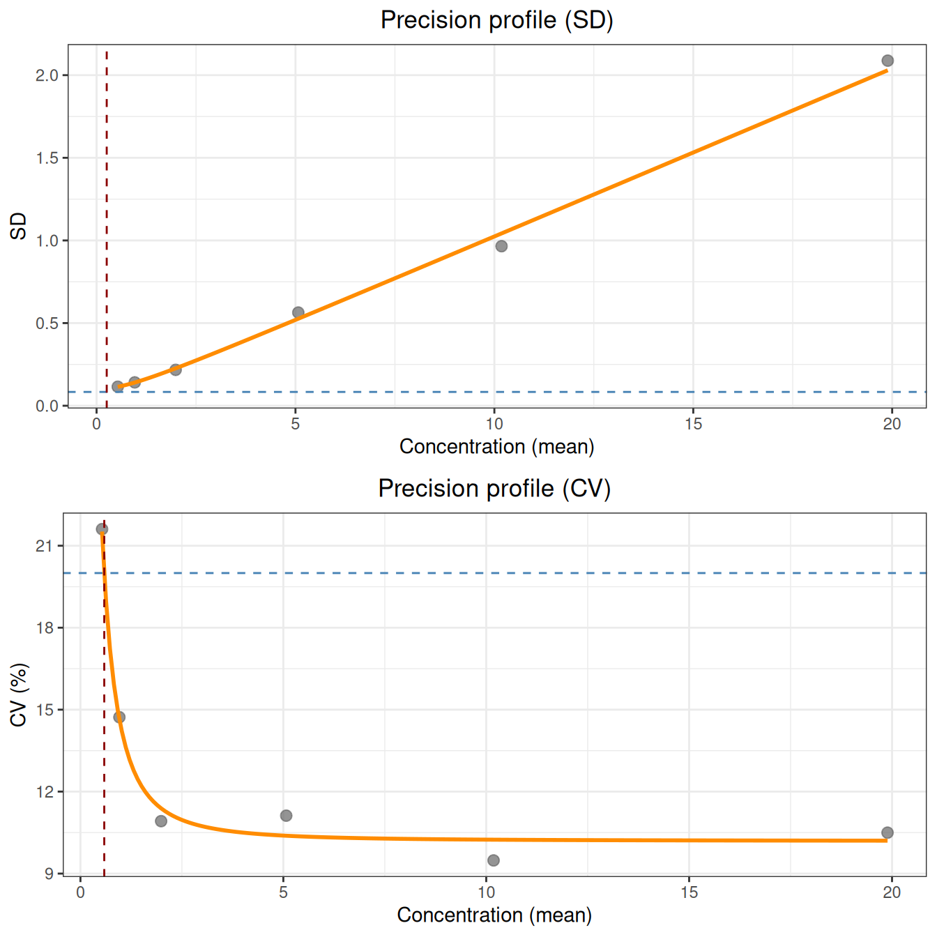
若无低浓度水平,则只计算 LoB,LoD / LoQ 为 NA:
res_b <- lob_lod_loq(summ[summ$sample %in% c("blank_A", "blank_B"), ],
                     sample_col = "sample", mean_col = "mean",
                     sd_col = "sd", n_col = "n",
                     blank = c("blank_A", "blank_B"))
res_b
Limit of Blank / Detection / Quantitation (EP17-A2)
LoB (parametric, B = 80, K = 2) : 0.08357
LoD (fixed-point) : --
LoQ (CV = 20%) : --
Note: LoQ is based on precision ONLY; bias is not included.若无空白样本(blank = NULL),则只计算 LoQ,LoB / LoD 为 NA:
res_q <- lob_lod_loq(summ[!summ$sample %in% c("blank_A", "blank_B"), ],
                     sample_col = "sample", mean_col = "mean",
                     sd_col = "sd", n_col = "n")
res_q
Limit of Blank / Detection / Quantitation (EP17-A2)
Precision profile: Sadler; best model = Model_3
Equation : sigma^2 = b1 + b2 * mu^2
Parameters : b1 = 0.010196, b2 = 0.010388
Fit : AIC = -479.4; RSS = 0.08315; GoF p = 0.9437
LoB (parametric, B = 0, K = 0) : --
LoD (fixed-point) : --
LoQ (CV = 20%) : 0.5868
Note: LoQ is based on precision ONLY; bias is not included.当按目标 CV 算出的 LoQ 低于 LoD 时(如空白噪声大、低浓度端精密度好),LoQ 会取 max(LoQ, LoD) 并以警告提示,保证 LoQ ≥ LoD:
# 构造"空白噪声大、低浓度精密度好"的数据
d_noisy <- data.frame(
  sample = c("blank", paste0("L", 1:6)),
  mean   = c(0, 0.5, 1, 2, 5, 10, 20),
  sd     = c(5, sqrt(0.01 + 0.02 * c(0.5, 1, 2, 5, 10, 20)^2)),
  n      = c(30L, rep(5L, 6))
)
res_n <- lob_lod_loq(d_noisy, sample_col = "sample", mean_col = "mean",
                     sd_col = "sd", n_col = "n", blank = "blank")
res_n
Limit of Blank / Detection / Quantitation (EP17-A2)
Precision profile: Sadler; best model = Model_3
Equation : sigma^2 = b1 + b2 * mu^2
Parameters : b1 = 0.01, b2 = 0.02
Fit : AIC = -469.2; RSS = 2.924e-29; GoF p = 1
LoB (parametric, B = 30, K = 1) : 8.261
LoD (fixed-point) : 10.79
LoQ (CV = 20%) : 10.79
Note: LoQ is based on precision ONLY; bias is not included.
Note: LoQ (precision) < LoD; LoQ reported as LoD = 10.79.cp 含 B−K 自由度修正,样本量小时不可忽略。max。lob_lod_loq() 的输入为已汇总 data.frame,原始的重复测量数据需先由replicate_to_mean()处理。